RUNS TEST OU TESTE DE RUNS OU TESTE DAS SEQUÊNCIAS

RESUMO

Você encontra aqui: a definição de run ou sequência; o teste de runs para 

verificar se uma sequência de dados é aleatória; o teste de runs para verificar 

a aleatoriedade da amostra; e o procedimento para o teste de runs em uma amostra.

                                                                    INTRODUÇÃO

Os exemplos estão simplificados. Para sequências maiores e mais complexas, o teste de runs pode ser calculado usando software estatístico.

 

DISTRIBUIÇÃO DE POISSON

                                                                                    

RESUMO

 Você encontra aqui: o que é distribuição de Poisson; função de probabilidade

 da distribuição de Poisson; usos da distribuição de Poisson; 

média e variância da distribuição; aproximação da distribuição de Poisson

 pela distribuição normal; aproximação da distribuição binomial

 pela distribuição de Poisson; aditividade da distribuição de Poisson.

INTRODUÇÃO

    

Exemplo

 

Lema de Neyman-Pearson

RESUMO

 Aqui se explica o que diz o lema de Neyman-Pearson. 

Para entender, você precisa conhecer os seguintes conceitos:

 hipótese nula; hipótese alternativa; nível de significância; 

poder do teste; teste de razão de verossimilhanças.

     LEMA DE NEYMAN-PEARSON

 

                                 We love feedback

                                 How would you rate your experience?

                           

Hypothesis Tests on a Single Standard Deviation

                     📌  Chi-square distribution

If Z is a random variable with a standardized normal distribution (mean zero and variance 1), then Z² has a chi-square distribution with 1 degree of freedom. 

 Z ∩ N (0,1)  Þ Z² ∩ c² (1df)

If Z₁, Z₂, ……, Z_k, are a set of independent and identically distributed standard normal variables, then the sum of their squares has a chi-square distribution with k degrees of freedom. 

                                                

Let X_i be k independent and normally distributed random variables with mean µ and variance σ²

 1. Then (X_i - µ), i from 1 to k, has mean zero and Σ (X_i - µ)² has a chi-square distribution with k degrees of freedom.

                               

                                                   🤯   EXAMPLE

In a city where police officers rely on speed radars that require regular calibration, a specialized center ensures that these devices operate correctly. Experts at the center have established that, in an urban area, radar speed readings (X_i) follow a normal distribution with a mean of 25 mph and a standard deviation of 3 mph:

·     Mean: μ = 25 mph

·     Standard deviation: σ = 3 mph

The manager of the center is considering purchasing new radars and has received proposals from two manufacturers. Both manufacturers claim that their radars produce speed readings that are normally distributed with a mean of 25 mph and a standard deviation of 1 mph.

🛑 Testing the First Manufacturer

To test the first manufacturer's claim, the manager instructs a technician to take five speed measurements using a test car programmed to travel exactly at 25 mph. The recorded speeds are:

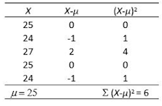
                                                    25, 24, 27, 25, 24

At a significance level of α = 10%, the null hypothesis is H₀: σ = 1 (the radar's standard deviation is 1 mph, as claimed.).

To test this claim, we calculate the variance:

                                                                              

The sum of squared deviations from the mean, ∑ (Xi − μ)² = 6. For a significance test at α = 10% with 5 degrees of freedom, the chi-square critical values are obtained. The calculated chi-square value of 6 falls within the acceptance region.

Conclusion: Since the calculated chi-square value of 6 falls within the acceptance region, the null hypothesis cannot be rejected. Then, the claim that the radar has a standard deviation of 1 mph is accepted. The first manufacturer's radar appears to be properly calibrated in terms of variance.

                                          🛑  Testing the Second Manufacturer

A second radar is tested under identical conditions. The recorded speeds are:

                                                              28, 27, 30, 28 ,29

If the radar readings are assumed to be normally distributed with a mean of 25 mph, we test the claim H₀: σ = 1.

Let's calculate the variance of X :

The upper critical chi-square value for α = 10% and 5 degrees of freedom is 11.07. Since the calculated sum of squared deviations (63) exceeds the upper critical value, it falls in the rejection region.

The  null hypothesis is rejected at the 10% significance level, indicating that the assumed variance does not hold. The second radar does not meet the claimed standard deviation of 1 mph, suggesting it is unreliable.

                        🛑 Reevaluating the Second Radar Using Sample Mean

While the variance test suggests the radar is unreliable, another issue is whether the radar is correctly measuring 25 mph. Instead of using the assumed mean (μ = 25 mph), we calculate the sample mean:

Conducting a hypothesis test for mean:

Using the known standard deviation (σ = 1 mph) and sample size (n =5), we can conduct a hypothesis test for the mean , applying the z-test :

where

Then, we have:

The critical z-value at α = 10%  is 1.645.

Since 7.60 is far beyond the critical z-value, we reject H₀. This confirms that the second radar is not correctly calibrated, as its mean is significantly different from 25 mph.

However, we could also calculate the sample variance, instead of using the assumed variance ((σ = 1 mph), and apply the t-test:

Let's calculate the variance of X :

The critical t-value at α = 10% and 4 degrees of freedom is 1.533.

Since 6.67 is far beyond the critical z-value, we reject H₀. This confirms that the second radar is not correctly calibrated, as its mean is significantly different from 25 mph.

                                                     ✅ Final Decision

·     The first manufacturer's radar passes the variance test and seems to be properly calibrated.

·     The second manufacturer's radar fails both the variance and mean tests, indicating a significant calibration error.

Recommendation: The center should accept the first manufacturer's radar and reject the second one due to its inaccuracy in measuring speed correctly.

Normal distribution: exercises

The graphical representation of a normal distribution is a bell-shaped curve that is symmetrical about the mean. Thus, half of the values ​​of the random variable X are equal to or greater than the mean and half are equal to or less than the mean. The curve covers 100% of the population. All possible values ​​that the random variable can assume lie under the curve. A normal distribution is defined by two parameters: the mean, denoted by µ and the standard deviation, denoted by σ.

Graphical representation of the

 normal distribution

🔴 EXERCISES

1.   On a certain road, the speed limit is 40 km/h with a tolerance of 7 km/h. The speed at which the driver travels on this road varies, with an average speed μ=40km/h and a standard deviation σ = 4 km/h. What is the probability that the driver will exceed 47 km/h and get a ticket? To determine this, we must standardize the variable (µ = 0, σ =1. Then we can consult a standardized normal distribution table, typically located at the end of statistical textbooks. Calculate:

Graphical representation of the

 decision rule

Tip: You can utilize software to determine probabilities.

2. In regular operation conditions, radar readings is a random variable normally distributed with mean μ = 25 mph and standard deviation σ = 3 mph. To test the calibration of the radar, a test car traveling at 25 mph is used. Assuming the radar is correctly calibrated, i.e., with μ = 25 mph and σ = 3 mph, what is the probability that the radar detects the test car's speed to be: a) 28 mph or higher? b) 27½ mph or higher? c) At what speed should the radar record for the probability of a value exceeding this speed to be 5%?

    a) Probability of detecting 28 mph or more.

                      b) Probability of detecting 27½ mph or more.

 c) To have a 5% probability of the radar measuring a higher speed.

     💡 TIP: More control means fewer mistakes. Compare probabilities  obtained in examples 2b,  3, 4.

3.  A calibration test will be carried out on 4 radars that operate together. A test car with a speed set at 25 mph will be used.  Under optimal conditions, the speed of each radar is a random variable following a normal distribution with mean µ=25 mph and standard deviation σ=3mph. If the radars are calibrated, what is the probability that the collected measurements will give an average speed of 27½ mph or higher?

Graphical representation 

average speed 27½ or more

4. The idea of ​​using 4 radars is good; however, having 9 is advantageous. Increased control (in this case, through a larger quantity of radars) decreases the risk of error. There are 9 calibrated radars in operation simultaneously. After calibration, the speed of each radar unit is a normally distributed random variable with mean µ = 25 mph and standard deviation σ = 3 mph. Using a test car traveling at a constant speed of 25 mph, what is the probability that the collected measurements will yield an average speed 27½ mph or higher?

              💡  TIP: If X and Y are independent random variables with                                   means µ₁ and µ₂ and variances σ₁² and σ₂² respectively, then:

          Z = X+Y is a random variable with mean µ₁+µ₂ and variance σ₁² + σ₂²

         W = X-Y is a random variable with mean µ₁-µ₂ and variance σ₁² + σ₂²·

          Var (a Z) = a² Var (Z)

           σ (a Z) = a σ (Z). 

5. If we consider the subway arrival time as a random variable with mean µ₁ = 8h10m and standard deviation σ₁ = 40s, and your arrival at the station as a random variable with mean µ₂ = 8h08m and standard deviation σ₂ =30s, how likely is it that you will miss the train? Let S represent the subway arrival time and Y represent your arrival time at the station. Therefore, W = S - Y, your waiting time, is a random variable with a normal distribution, having an average of 8:10 – 8:08 = 2 m = 120 s, variance of 402 + 302 =1600 + 900 = 2500 s, and a standard deviation of 50. Missing the train would occur if W ≤ 0. To calculate the probability of W ≤ 0:

Graphical representation of decision rule

💡 Set critical values ​​ to reject specific results. The decision rule is crucial for quality control.     

6. In the canning industry, the pH (the acidity) of the product in each can is a random variable that is normally distributed with mean 7 and standard deviation of 0.5. If the pH of the product falls below 6.0 or exceeds 8.0, the can is rejected. What is the probability of this happening?