This is one of the most frequent questions asked by those
starting to analyze data:
“Do my data need to be
normally distributed?”
Let’s clarify:
To apply analysis of variance (ANOVA), it is not necessary
for the data themselves to follow a normal distribution.
What is required is that the residuals (or errors) from the
ANOVA model are approximately normally distributed.
🔍 What are residuals?
A residual is the difference between an observed value and
the mean of the group it belongs to.
In a one-way ANOVA, the residual is calculated as:
Residual =
observed value – group mean
📊 Example:
Imagine the data shown in Table 1. The group means are
listed at the bottom of the table.
Table 1– Data from a trial
Based on these values, we calculate the residuals by
subtracting the group mean from each data point.
Table 2 – Residuals
📈 Why analyze residuals?
The study of residuals — called residual analysis — is
crucial because ANOVA assumes that residuals are normally distributed.
That’s why we always need to analyze the residuals when
using ANOVA.
🧪 How do we analyze
residuals?
A good practice is to examine residuals graphically and use
statistical tests to verify that ANOVA assumptions are met. Figure 1 shows the
histogram from Table 2 residuals.
Figure
1. Histogram of residuals
Symmetry is a good sign. ANOVA is robust to minor violations of normality, especially when residuals are approximately symmetric. Figure 2 shows the boxplot of the residuals.
Figure 2. Boxplot
Symmetry and absence of outliers strengthen the case that
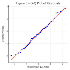
ANOVA assumptions are satisfied. The Q-Q plot (quantile-quantile) compares
observed residuals to what would be expected under normality. If points align
along a 45° line, that’s a good sign. The P-P plot is another visual tool to
assess normality.
📌 Descriptive statistics of
residuals
Some summary measures help evaluate the distribution:
■ Mean and median: If equal or close →
symmetry
■
Skewness coefficient: Close to zero → good
■
Kurtosis: Negative values suggest a flatter distribution, which is not
necessarily problematic
Table 3 –
Descriptive statistics of residuals
In our example:
■ Mean =
0
■ Median
= 0
· Skewness = 0 (symmetric)
· Slightly negative kurtosis (light tails), but still acceptable
✅ Statistical tests of
normality
Normality tests
provide objective checks. The most common ones include:
■Shapiro-Wilk
■ Kolmogorov-Smirnov
In our example, the Kolmogorov-Smirnov test was performed
in SPSS and resulted in p = 0.200.
That means there is no evidence to reject normality of the
residuals.
⚠️ A note on sample size:
■ Small samples: less power to detect
non-normality.
■ Large
samples: may detect minor deviations that don't impact ANOVA results.
🧠 Final thoughts:
■ When group sizes are equal and fixed
factors are used, ANOVA remains reliable despite slight violations of
normality.
■
Problems arise mainly with high skewness or very different group variances.
💡
Important takeaway:
Raw data are usually not normally distributed, because they
come from distinct groups expected to have different means.
What matters is:
➤ Whether the residuals follow
a normal distribution, or
➤ Even better, whether each group’s data
is normally distributed.
💡 Summary
🔴 When Violations of Assumptions Are Problematic for ANOVA
- Non-Normal
Distributions (especially Kurtosis):
- Leptokurtic
distributions (heavy-tailed): The F-test becomes too
conservative, leading to a loss of statistical power. It fails to detect real effects.
- Platykurtic
distributions (light-tailed): The F-test becomes too
liberal, inflating the Type I error rate. It may find "significant" effects that are not real.
- Heteroscedasticity
(Skewed Distributions): As you correctly stated, variance often
increases with the mean in skewed data. This heteroscedasticity can
seriously bias the F-statistic and invalidate the results.
🟢 When
the F-test is Robust to Violations
- Equal sample
sizes across groups.
- Large samples.
📚 References:
1. Ghasemi, A. & Zahediasl, S. (2012). Normality Tests
for Statistical Analysis: A Guide for Non-Statisticians. Int J Endocrinol
Metab. 10(2): 486–489.
2. Scheffé, H. (1959). The Analysis of Variance. Wiley.


No comments:
Post a Comment