The Importance of Resolution in Evaluating Measurement Uncertainty

Resolution is the smallest variation that can be detected by a measuring instrument. For example, a measuring tape with markings every 1 cm has a resolution of 1 cm — meaning it registers changes in 1 cm increments.

Resolution represents the smallest measurable increment: it is the minimum difference that can produce a detectable change in the reading.

If you try to measure the diameter of a keyhole using a measuring tape, you will get the same result every time — even after 100 repetitions — because the resolution of the tape is not sufficient to detect such small variations.

Exemples:

       ·        If the instrument measures in 1-unit steps, any value between 6.5 and 7.5 will be recorded as 7.                                                                                 

                                                                              

        ·        If it measures in 2-unit steps, values between 7 and 9 will be recorded as 8.

  

🔎 Measurement Uncertainty

In a previous post (Type B Evaluation of Measurement Uncertainty), we explained that a measurement should be reported as:

                                                         (X ± ΔX) unit

Where:

             ·        X is the best estimate of the measured value;

             ·        ΔX is the associated uncertainty.

This means that if the measurement is repeated under the same conditions, the result is expected to fall within the range:

                                                 (X - ΔX) to (X + ΔX)

To evaluate the uncertainty of a single measurement, it is essential to consider the resolution of the instrument used.

---

👶 Example: length of a newborn

Suppose you know only that a newborn measured 50 cm in length. That information alone is not enough to estimate the uncertainty.

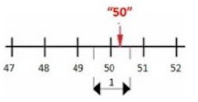
However, if you also know that the measurement was taken using a ruler graduated in centimeters, you can state that the actual length was between 49.5 cm and 50.5 cm. The result should be expressed as:

                                                          (50.0 ± 0.5) cm

In this case, the uncertainty arises solely from the instrument’s limitation, assuming it is properly calibrated. Because only one measurement was taken, the uncertainty is not statistical and is classified as Type B.

 

---

⚖️ Example: mass of the newborn

Now suppose the scale used has divisions every 10 g (0.01 kg). If the reading is 3.54 kg, the actual mass is between 3.535 kg and 3.545 kg.

This measurement should be written as:

                                                           (3.54 ± 0.005) kg

---

📐 Absolute and Relative Uncertainty

In the expression X ± ΔX, the term ΔX is called the absolute uncertainty (formerly known as the absolute error).

Relative uncertainty tells us how significant the absolute uncertainty is compared to the measured value. It is calculated as:

---

🚗 Example: speedometer reading

Let’s say a car speedometer is marked in increments of 2 km/h. If you read 60 km/h:

             ·        The absolute uncertainty is half the smallest division: 1 km/h

             ·        The relative uncertainty is:

Relative uncertainty is dimensionless, because the units cancel out. This makes it especially useful for comparing the precision of different physical quantities.

---

📊 Example: mass or length?

Back to the newborn: which measurement had greater uncertainty?

     Length:

     Mass:

➡️ The length measurement had greater relative uncertainty.

---

These definitions apply to Type B uncertainty, but are equally valid in the context of Type A uncertainty, which is based on statistical analysis.

---

✏️ Practice Exercises

          1.     You measured a child’s height with a ruler graduated in centimeters and got 80            cm. What is the uncertainty?

          2.     You measured a child’s temperature with a thermometer marked in 2 °C                       increments and got 38 °C. What is the uncertainty?

✅ Answers

            1.     Height = (80 ± 0.5) cm
            Relative uncertainty = (0.5 / 80) × 100 = 0.625%

           2.     Temperature = (38 ± 1) °C
            Relative uncertainty = (1 / 38) × 100 = 2.63%

---

Do My Data Need to Be Normally Distributed to Use ANOVA?

This is one of the most frequent questions asked by those starting to analyze data:

“Do my data need to be normally distributed?”

Let’s clarify:

To apply analysis of variance (ANOVA), it is not necessary for the data themselves to follow a normal distribution.

What is required is that the residuals (or errors) from the ANOVA model are approximately normally distributed.

🔍 What are residuals?

A residual is the difference between an observed value and the mean of the group it belongs to.

In a one-way ANOVA, the residual is calculated as:

                           Residual = observed value – group mean

📊 Example:

Imagine the data shown in Table 1. The group means are listed at the bottom of the table.

                                                         Table 1– Data from a trial

Based on these values, we calculate the residuals by subtracting the group mean from each data point.
                                                         Table 2 – Residuals

📈 Why analyze residuals?

The study of residuals — called residual analysis — is crucial because ANOVA assumes that residuals are normally distributed.

That’s why we always need to analyze the residuals when using ANOVA.

🧪 How do we analyze residuals?

A good practice is to examine residuals graphically and use statistical tests to verify that ANOVA assumptions are met. Figure 1 shows the histogram from Table 2 residuals.

                                          Figure 1. Histogram of residuals

Even if it’s not a “perfect normal distribution,” note the symmetry — this is a good sign. ANOVA is robust to minor violations of normality, especially when residuals are approximately symmetric. Figure 2 shows the boxplot of the residuals. 

Figure 2. Boxplot

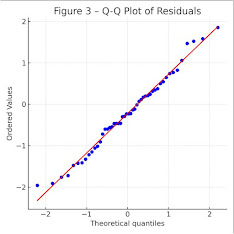
Symmetry and absence of outliers strengthen the case that ANOVA assumptions are satisfied. The Q-Q plot (quantile-quantile) compares observed residuals to what would be expected under normality. If points align along a 45° line, that’s a good sign. The P-P plot is another visual tool to assess normality.

                                                 Figure 3 – Q-Q plot of the residuals

                                       

📌 Descriptive statistics of residuals

  Some summary measures help evaluate the distribution:

■ Mean and median: If equal or close → symmetry
■ Skewness coefficient: Close to zero → good
■ Kurtosis: Negative values suggest a flatter distribution, which is not necessarily problematic

                     Table 3 – Descriptive statistics of residuals

                                    

In our example:
■ Mean = 0
■ Median = 0
· Skewness = 0 (symmetric)
· Slightly negative kurtosis (light tails), but still acceptable

✅ Statistical tests of normality

    Normality tests provide objective checks. The most common ones include:
              ■Shapiro-Wilk
              ■ Kolmogorov-Smirnov

In our example, the Kolmogorov-Smirnov test was performed in SPSS and resulted in p = 0.200.

That means there is no evidence to reject normality of the residuals.

⚠️ A note on sample size:

■ Small samples: less power to detect non-normality.
■ Large samples: may detect minor deviations that don't impact ANOVA results.

🧠 Final thoughts:

■ When group sizes are equal and fixed factors are used, ANOVA remains reliable despite slight violations of normality.
■ Problems arise mainly with high skewness or very different group variances.

💡 Important takeaway:

Raw data are usually not normally distributed, because they come from distinct groups expected to have different means.

What matters is:

➤ Whether the residuals follow a normal distribution, or
➤ Even better, whether each group’s data is normally distributed.

📚 References:

1. Ghasemi, A. & Zahediasl, S. (2012). Normality Tests for Statistical Analysis: A Guide for Non-Statisticians. Int J Endocrinol Metab. 10(2): 486–489.
2. Scheffé, H. (1959). The Analysis of Variance. Wiley.

When Unequal Variances Matter in ANOVA — and When They Don’t

 

🔴 When the violation of homoscedasticity affects ANOVA

     1. Positive kurtosis (above 2): the F test loses power. That is, it tends not to reject the null hypothesis, even when it is false.
     2. Skewed distributions: in this case, variance tends to increase with the mean, which can seriously bias ANOVA results.

🟢 When the violation does not seriously compromise the analysis

     1. Equal sample sizes across groups: if the groups have the same number of observations (r₁ = r₂ = ... = rₖ), small differences in variances are usually acceptable — unless one is highly discrepant.
     2. Large samples: with more than 10 observations per group, the F test tends to remain robust to mild heteroscedasticity.

How to test the homogeneity of variances?

 The goal is to test the null hypothesis:
                      H₀: s²₁ = s²₂ = s²₃ = ... = s²ₖ (i = 1, 2, ..., k)

against the alternative that at least one variance is different.

Among the available tests, we highlight:
     · Levene’s test ✅
     · Bartlett’s test ⚠️
     · Cochran’s test and Hartley’s test (less common)

⚠️ Beware of Bartlett’s test:
It may mask differences in platykurtic distributions and indicate spurious differences in leptokurtic ones.

Understanding Levene’s Test

Levene’s test evaluates whether the groups have similar dispersions. The logic is simple: if the groups have homogeneous variances, the residuals (or their transformations) should not differ significantly.

✔️ Traditional procedure (with squared residuals)

     1. Calculate the residuals.
     2. Square these residuals.
     3. Perform a new one-way ANOVA using the squared residuals as the variable.

❗ If the F value is not significant, homoscedasticity is assumed.

    EXAMPLE

                                                                   Table 1 – Raw data by group

Table 2 – Squared residuals

Table 3 – Levene’s test result (SAS output)

✔️ Practical alternative (using absolute residuals)

      Another version of Levene’s test — more common in software like SPSS — uses the absolute                values of residuals instead of squares.

      ❗ The procedure is the same: perform an ANOVA using the absolute values.

📊 Table 4 – Levene’s test result (SPSS output)

📌 Note: The F values may differ slightly, but the conclusion is the same — here, there is no evidence of heteroscedasticity.

✔️ Alternative versions:
It is also possible to compute residuals based on the trimmed mean or the median, which may make the test more robust to outliers.

When homoscedasticity fails: what to do?

If the hypothesis of equal variances is rejected, the classic ANOVA may be inappropriate. But there are alternatives:

1. Data transformations
They can stabilize variances and make the data more normally distributed:
· Logarithmic (for positive, skewed data)
· Square root (ideal for counts)
· Arcsine square root (for proportions)
· Standardization (z-scores)

2. Nonparametric tests
· Kruskal-Wallis: replaces ANOVA when assumptions are not met.

3. Other solutions
· Remove outliers, if justified
· Increase sample size
· Redesign the experiment

💡 In summary:

The homogeneity of variances is a key assumption of ANOVA, but its violation is not always fatal. Understanding your data, choosing the right test, and interpreting the results carefully are essential attitudes for any good researcher.

References:

1. Dean, A. & Voss, D. (1999). *Design and Analysis of Experiments*. Springer.
2. Scheffé, H. (1959). *The Analysis of Variance*. Wiley.
3. Zaiontz, C. Levene’s test. Retrieved from http://www.real-statistics.com/one-way-analysis-of-variance-anova/homogeneity-variances/levenes-test/

4. And, why not?